In real-world programming, writing an algorithm is not enough, and proving that it is efficient is the key. Big O notation allows us to easily categorize the efficiency of a given algorithm and convey it to others. From a mathematical perspective, Big O describes the upper bound of the growth rate of a function.
Big O notation owes its name to its simplicity and elegance, borrowed from the German word “Ordnung” or “order”. Introduced by Paul Bachmann (a German mathematician) and later widely used by Donald Knuth (father of the analysis of algorithms), the Big O describes the behavior of various mathematical functions as their inputs grow infinitely.
1. The Big O Notation
At its core, Big O notation provides a way to express the upper bound on the growth rate of an algorithm’s resource consumption (usually time or space) concerning the size of its input. The notation is expressed as ‘O(f(n))’, where ‘f(n)‘ represents a mathematical function that characterizes the algorithm’s resource usage in relation to the input size ‘n‘.
At a broad level, the Big O notation signifies how will an algorithm’s performance change as the data increases.
During application development using Big O, we can calculate how much time should be allocated for processing a certain amount of input data and be sure that the algorithm will process it within the allotted time. In runtime, an algorithm might sometimes work even better than what the Big O notation shows for its complexity, but not worse.
2. An Analogy
Imagine that we have a race where runners compete against each other to win. But there is a catch: the race course has no finish line. Since the race is infinite, to win a race a runner has to surpass the other slower opponents over time and not finish first.
Now in the above analogy, replace the runners with algorithms and race track distance is our algorithm input. How far from the start a player runs, after a certain amount of time, represents the amount of work done by the algorithm.
Different algorithms will demonstrate different performances as the race continues (input grows). Some algorithms will perform faster than others for small inputs, but degrade performance as the input grows, although it never stops moving. Similarly, some algorithms will perform consistently no matter the size of the input.
Note that the efficiency of each algorithm is always evaluated in the long run.
3. An Example
Suppose we have two functions in Python that find the maximum element in an array.
The first function, ‘find_max_element_linear‘ function uses a linear search to find the maximum element in the array. It iterates through the entire array once to find the max element.
def find_max_element_linear(arr):
  max_element = arr[0]
  for element in arr:
    if element > max_element:
      max_element = element
  return max_element
This function performs a constant number of operations (comparisons and assignments). The number of iterations is directly proportional to the input size ‘n’.
To derive the Big O notation, we need to count the number of basic operations in the worst-case scenario. In this case, the worst-case scenario occurs when the largest element is at the end of the array, and the loop iterates through all elements. Therefore, the time complexity is O(n), where ‘n’ represents the size of the input array.
In the context of Big O notation, we express this algorithm’s time complexity as O(n) because it grows linearly with the input size. This means that as the size of the array doubles, the number of operations required also approximately doubles.
The second function ‘find_max_element_constant‘ utilizes Python’s built-in max function which is designed for finding the maximum element in a sequence. This function has a time complexity of O(1) since it doesn’t depend on the size of the array but only returns the maximum element directly.
def find_max_element_constant(arr):
  max_element = max(arr)
  return max_element
The key differentiator is the ‘max’ function. Since the max function’s execution time does not depend on the input size ‘n’, it is considered constant time. Because of this, the ‘find_max_element_constant’ also operates in constant time, regardless of the size of the input array.
In the context of Big O notation, this algorithm’s time complexity is O(1) because it exhibits constant behavior. So no matter how much the input size grows, the number of operations required by the ‘find_max_element_constant’ function remains the same.
4. Commonly Used Big O Notations
Algorithms are classified into different complexity classes, such as O(1), O(log n), O(n), O(n log n), O(n^2), and more. Let’s take a closer look at some of these.
It is worth noting, that in practical terms, an algorithm with worse theoretical complexity might perform better for small inputs due to optimizations. However, Big O notation helps us understand how an algorithm behaves as the input size approaches infinity.
4.1. O(1) Constant Time
An algorithm has constant time complexity if its execution time or the number of operations it performs remains constant and does not depend on the input size. The number of operations can be one, two, twenty-six, or two hundred – it doesn’t matter. The important thing is that it doesn’t depend on the input size.
For example, accessing an element in an array by its index is done in constant time regardless of the array’s size.
4.2. O(n) Linear Time
An algorithm has linear time complexity (O(n)) when the number of operations is directly proportional to the size of the input. As the input size grows, the number of operations also grows linearly.
For example, iterating through an array to find a specific element. The time it takes to find the element increases linearly with the size of the array because you might have to examine each element.
4.3. O(log n) Logarithmic Time
An algorithm has logarithmic time complexity (O(log n)) when the number of operations grows in proportion to the logarithm of the input size. This means that as the input size increases, the number of operations increases slowly.
For example, binary search in a sorted collection. With each comparison, the search space is reduced by half, resulting in a time complexity that grows logarithmically as the input size increases.
4.4. O(n log n) Linearithmic/Log-linear Time
An algorithm has linearithmic time complexity (O(n log n)) when the number of operations grows in proportion to the product of the input size ‘n’ and the logarithm of ‘n.’ It falls between linear and quadratic complexity.
For example, efficient sorting algorithms like Merge Sort and Quick Sort. These algorithms divide the input into smaller parts and then combine them, resulting in a time complexity that is n times the logarithm of ‘n.’
4.5. O(sqrt(n)) Square Root Time
Square root time complexity means that the algorithm requires O(n^(1/2)) evaluations where the size of the input is n.
An example of an algorithm with square root time complexity is the binary search algorithm that is used to find the position of a target value in a sorted array. The algorithm works by repeatedly dividing the array in half and then searching the half that contains the target value.
4.6. O(2^n) Exponential Time
As per the mathematical concept, the number of subsets of a set of ‘n’ elements is equal to ‘2^n’, therefore, it is reasonable to expect that such algorithms scan all the subsets of the input elements. Such algorithms are extremely inefficient in practice, even for small input sizes.
For example, generating a Fibonacci series. To generate 15 Fibonacci numbers, there will be 32768 operations which can also be said as 2^15 operations. Thus an exponential time complexity.
In practice, exponential time complexity is often too slow to be used to solve real-world problems. However, it is still a valuable tool for theoretical computer science, and it is used to solve some important problems, such as the knapsack problem.
4.7. O(n^2) Quadratic Time
An algorithm has quadratic time complexity (O(n^2)) when the number of operations grows in proportion to the square of the input size. As the input size increases, the number of operations grows quadratically.
For example, the nested loops where we compare all pairs of elements in an array. As the array size increases, the number of comparisons grows quadratically with the number of elements.
4.8. O(n^k) Polynomial Time
In polynomial time complexity, the number of operations grows as a polynomial function of the input size ‘n’ with ‘k’ being a constant exponent. Polynomial time complexity is considered efficient, especially when ‘k’ is a small constant. However, as ‘k’ increases, polynomial time algorithms can still become impractical for large input sizes.
For example, algorithms like Floyd-Warshall for all-pairs shortest paths demonstrate the polynomial time complexity. The number of operations grows as a polynomial of the input size (number of vertices).
4.9. O(n!) Factorial Time
In these algorithms, the number of operations grows at an exponential rate as a factorial of the input size ‘n’. Factorial time complexity is rarely seen in practical algorithm design due to its impracticality for all except the smallest inputs.
For example, given a set of ‘n’ distinct elements, find all possible permutations (arrangements) of those elements. The algorithm tries all possible options for each position in the permutation, creating a tree of recursive calls. As a result, the number of recursive calls grows at a factorial rate with ‘n’.
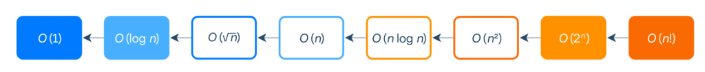
4.10. Ordering Complexities By Performance
Now let’s sort these notations from the best to the worst so that we remember which ones are the most effective, and which ones we should stay away from.
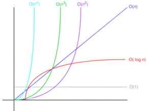
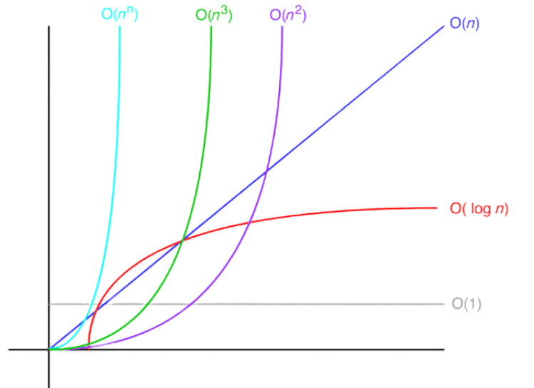
To visualize how some of these algorithms, see the next line chart which helps you visualize how the performance of algorithms changes as the input grows.
5. Difference between Time Complexity and Space Complexity
The big O notations are often associated with two types of complexities:
- time complexity
- space complexity
Let’s understand the difference between the both.
Time complexity refers to the amount of time an algorithm takes to complete its task as a function of the size of the input. It is typically measured in terms of the number of basic operations (such as comparisons, assignments, or arithmetic operations) executed by the algorithm in the worst-case, average-case, or best-case scenarios.
Time complexity helps assess how quickly an algorithm solves a problem concerning input size. It provides insights into an algorithm’s speed and efficiency.
Space complexity is the amount of memory or storage space an algorithm uses in addition to the input data to execute the task. It is measured in terms of the number of memory locations (or amount of memory) required by the algorithm in the worst-case, average-case, or best-case scenarios.
Space complexity helps assess how efficiently an algorithm utilizes memory resources. It is crucial in scenarios where memory is limited, such as in embedded systems or on devices with constrained resources.
Using Big O notations, the space complexity expresses an upper bound on the amount of memory used by the algorithm whereas the time complexity expresses how quickly an algorithm solves a problem. Both time and space complexity analysis are essential for designing and evaluating algorithms that are both fast and memory-efficient.
6. Conclusion
Big O notation represents the efficiency of an algorithm in relation to the size of its input. Algorithms are classified into different complexity classes and we learned about them in brief. Mastering Big O notation and understanding time and space complexity is crucial for building efficient algorithms, optimizing code performance, and ultimately delivering a better user experience.
Happy Learning !!